Lesson 2 Getting Our Project Organized
teaching: 20
exercises: 10
adapted from: http://swcarpentry.github.io/r-novice-gapminder/02-project-intro/index.html
questions:
- How do I actually begin coding in R?
- How to manage your environment?
- How to install packages?
objectives:
- Organize our new package directory
- Install additional packages using
install.packages()command - Create our first rmarkdown document
keypoints:
- Use RStudio to create and manage projects with consistent layout.
- Use
install.packages()to install packages (libraries).
2.0.1 Downloading the data and getting set up
For this lesson we will use the following folders in our working directory: data/, data_output/ and fig_output/. Let’s write them all in lowercase to be consistent. We can create them using the RStudio interface by clicking on the “New Folder” button in the file pane (bottom right), or directly from R by typing at console:
dir.create("data")
dir.create("data_output")
dir.create("fig_output")
2.1 Installing packages using the packages command
In addition to the core R installation, there are in excess of 10,000 additional packages which can be used to extend the functionality of R. Many of these have been written by R users and have been made available in central repositories, like the one hosted at CRAN, for anyone to download and install into their own R environment. In the course of this lesson we will be making use of several of these packages, such as ‘ggplot2’ and ‘dplyr’.
Additional packages can be installed from the command line or within a script.
2.1 Exercise
Use the console to install the tidyverse package. Find the console (bottom left pane) and type
install.packages("tidyverse")The ‘tidyverse’ package is really a package of packages, including ‘ggplot2’ and ‘dplyr’, both of which require other packages to run correctly. All of these packages will be installed automatically. Depending on what packages have previously been installed in your R environment, the install of ‘tidyverse’ could be very quick or could take several minutes. As the install proceeds, messages relating to its progress will be written to the console. You will be able to see all of the packages which are actually being installed.
Because the install process accesses the CRAN repository, you will need an Internet connection to install packages.
It is also possible to install packages from other repositories, as well as Github or the local file system, but we won’t be looking at these options in this lesson.
We will also need a package called knitr. > > install.packages("knitr") > > As the install proceeds, messages relating to its progress will be written to the console. You will be able to see all of the packages which are actually being installed.
2.2 Creating an R Markdown file
Within RStudio, click File → New File → R Markdown and you’ll get a dialog box like this: 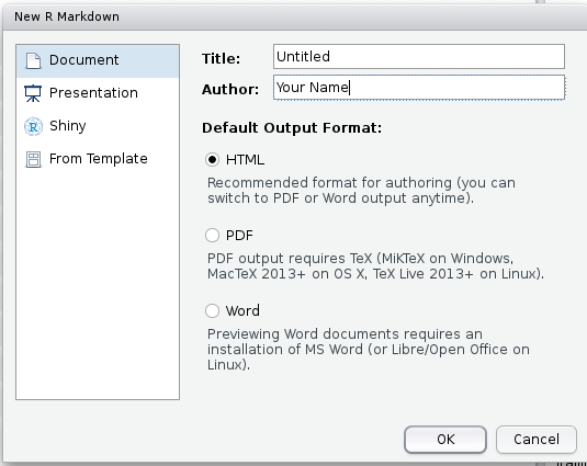
You can stick with the default (HTML output), but let’s call it “intro-to-r”.
2.3 Basic components of R Markdown
The initial chunk of text (header) contains instructions for R to specify what kind of document will be created, and the options chosen. You can use the header to give your document a title, author, date, and tell it that you’re going to want to produce html output (in other words, a web page).
---
title: "Initial R Markdown document"
author: "Karl Broman"
date: "April 23, 2015"
output: html_document
---
You can delete any of those fields if you don’t want them included. The double-quotes aren’t strictly necessary in this case. They’re mostly needed if you want to include a colon in the title.
RStudio creates the document with some example text to get you started. Note below that there are chunks like
```{r}
summary(cars)
```
These are chunks of R code that will be executed by knitr and replaced by their results. More on this later.
A quick preview of markdown formatting you can use before we delve in deeper tomorrow:
to add headers of various sizes, use:
# Title
## Main section
### Sub-section
#### Sub-sub section
You make things bold using two asterisks, like this: **bold**, and you make things italics by using underscores, like this: _italics_.
Go ahead and write this down for reference as we learn today.
Next, we will download the dataset needed for these lessons. We won’t be using this right away, but we want to be prepared for when we need it. I’ll paste this into the etherpad, but we will be entering a command to download a dataset from the internet to a specific destination.
download.file("https://ndownloader.figshare.com/files/11492171",
              "data/SAFI_clean.csv", mode = "wb")
Notice that this is being downloaded into our data folder. We can access that destination from our current working directory by including the data/ in front of the file name.