New Immigrant Destinations
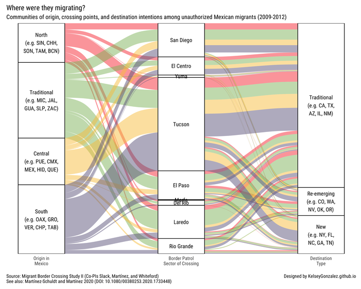
Using data from the Migrant Border Crossing Project (Slack, Martínez, and Whiteford), I map out how Mexican origins cross the US border at different points en route to new destinations. This visualization was created to support the new publication of “Destination Intentions of Unauthorized Mexican Border Crossers and Familial Ties to US Citizens” at The Sociological Quarterly.
knitr::opts_chunk$set(echo = TRUE,
                      results = "hide",
                      warning = FALSE,
                      message = FALSE)

if (!require("pacman")) install.packages("pacman")
## Loading required package: pacmanpacman::p_load(tidyverse, ggalluvial, readxl, ggrepel)load data
df <- readxl::read_excel("MBCS II_geo_3.xls") %>%
  drop_na() %>%
  mutate(across(state_mex:dest_type_us, ~ as.factor(.)),
         across(state_mex:census_region_us, ~ fct_recode(., NULL = "Don't Know")),
         region_mex = fct_relevel(region_mex,
                                  c("North", "Traditional", "Central", "South")),
         sector_cross = fct_relevel(sector_cross,
                                    c("San Diego","El Centro","Yuma", "Tucson",
                                      "El Paso","Marfa","Del Rio","Laredo","McAllen")),
         census_div_us = fct_relevel(census_div_us,
                                     c("Pacific","Mountain", "West South Central",
                                       "West North Central", "East South Central",
                                       "East North Cenral",  "South Atlantic",
                                       "Mid-Atlantic", "New England")),
         census_region_us = fct_relevel(census_region_us,
                                        c("West", "South", "Midwest", "Northeast")),
         dest_type_us = fct_relevel(dest_type_us,
                                    c("Traditional","Re-Emerging","New Destination")),
         sector_cross = fct_recode(sector_cross, "Rio Grande" = "McAllen")) %>%
  select(region_mex, sector_cross, dest_type_us, census_div_us, census_region_us) %>%
  drop_na()
add descriptors to labels
mex_states <- tibble::tribble(
  ~state_mex, ~state_mex_abbreviation, ~state_mex_code, ~state_mex_3code,
  "Aguascalientes", "Ags.","AG","AGU",
  "Baja California", "B.C.","BC","BCN",
  "Baja California Sur", "B.C.S.","BS","BCS",
  "Campeche","Camp.","CM","CAM",
  "Chiapas","Chis.","CS","CHP",
  "Chihuahua","Chih.","CH","CHH",
  "Coahuila","Coah.","CO","COA",
  "Colima", "Col.","CL","COL",
  "DF", "CDMX","DF","CMX",
  "Durango", "Dgo.","DG","DUR",
  "Guanajuato", "Gto.","GT","GUA",
  "Guerrero", "Gro.","GR","GRO",
  "Hidalgo", "Hgo.","HG","HID",
  "Jalisco", "Jal.","JA","JAL",
  "Mexico","Edomex.","EM","MEX",
  "Michoacan","Mich.","MI","MIC",
  "Morelos", "Mor.","MO","MOR",
  "Nayarit", "Nay.","NA","NAY",
  "Nuevo Leon", "N.L.","NL","NLE",
  "Oaxaca", "Oax.","OA","OAX",
  "Puebla", "Pue.","PU","PUE",
  "Queretaro", "Qro.","QT","QUE",
  "Quintana Roo","Q. Roo.","QR","ROO",
  "San Luis Potosi", "S.L.P.","SL","SLP",
  "Sinaloa", "Sin.","SI","SIN",
  "Sonora", "Son.","SO","SON",
  "Tabasco", "Tab.","TB","TAB",
  "Tamaulipas", "Tamps.","TM","TAM",
  "Tlaxcala","Tlax.","TL","TLA",
  "Veracruz", "Ver.","VE","VER",
  "Yucatan", "Yuc.","YU","YUC",
  "Zacatecas", "Zac.","ZA","ZAC"
)

add_ex <- function(state){
  df <- readxl::read_excel("MBCS II_geo_3.xls")  %>%
    left_join(mex_states, by = "state_mex") %>%
    count(region_mex, state_mex, state_mex_3code) %>%
    filter(region_mex == state) %>%
    arrange(desc(n)) %>%
    top_n(5, n) %>%
    pull(state_mex_3code)
  string <- str_wrap(
    paste0(
      "(e.g. ",
      paste(df, collapse = ", "),
      ")"),
    18)
  df <- paste0(state,"\n", string)
  return(df)
}

North <- add_ex("North")
Traditional <- add_ex("Traditional")
Central <- add_ex("Central")
South <- add_ex("South")
Add in labeled names to dataset, reorder the region_mex factors from North to South.
df <- df %>%
  mutate(region_mex_named = as.character(region_mex),
         region_mex_named = case_when(region_mex_named == "North" ~ North,
                                      region_mex_named == "Traditional" ~ Traditional,
                                      region_mex_named == "Central" ~ Central,
                                      region_mex_named == "South" ~ South),
         region_mex_order = case_when(region_mex == "North" ~ 1,
                                      region_mex == "Traditional" ~ 2,
                                      region_mex == "Central" ~ 3,
                                      region_mex == "South" ~ 4),
         region_mex_named = fct_reorder(region_mex_named, region_mex_order),
         dest_type_us_named = fct_recode(dest_type_us,
                                         "Traditional\n(e.g. CA, TX,\nAZ, IL, NM)" = "Traditional",
                                         "Re-emerging\n(e.g. CO, WA,\nNV, OK, OR)" =  "Re-Emerging",
                                         "New\n(e.g. NY, FL,\nNC, GA, TN)" = "New Destination")) %>%
  select(region_mex_named, sector_cross, dest_type_us_named, census_div_us, census_region_us)
And, plot!
ggplot(data = df,
       aes(axis1 = region_mex_named,
           axis2 = sector_cross,
           axis4 = dest_type_us_named)) +
  scale_x_discrete(limits = c("Origin in\nMexico",
                              "Border Patrol\nSector of Crossing",
                              "Destination\nType"),
                   expand = c(.1, .05)) +
    scale_y_continuous(expand = c(0,0)) +
  geom_alluvium(aes(fill = region_mex_named), show.legend = FALSE, stat='flow') +
  geom_stratum() +
  geom_text(stat = "stratum", family = "Roboto Condensed",aes(label = after_stat(stratum))) +
  scale_fill_manual(values = c("#f94144", #red
                               "#90be6d", #green
                               "#f9c74f", #yellow
                               "#70688d" #purple
                               )) +
  ggtitle("Where were they migrating?",
          subtitle = "Communities of origin, crossing points, and destination intentions among unauthorized Mexican migrants (2009-2012)") +
  labs(caption = c("
                   Designed by KelseyGonzalez.github.io",
                    "
Source: Migrant Border Crossing Study II (Co-PIs Slack, Martínez, and Whiteford)
See also: Martínez-Schuldt and Martínez 2020 (DOI: 10.1080/00380253.2020.1733448)")) +
      theme_minimal(base_family = "Roboto Condensed", base_size = 12) +
  theme(axis.text.y = element_blank(),
        axis.ticks = element_blank(),
        panel.grid = element_blank(),
        plot.margin = margin(10, 10, 10, 10),
plot.caption = element_text(hjust=c(1, 0))) 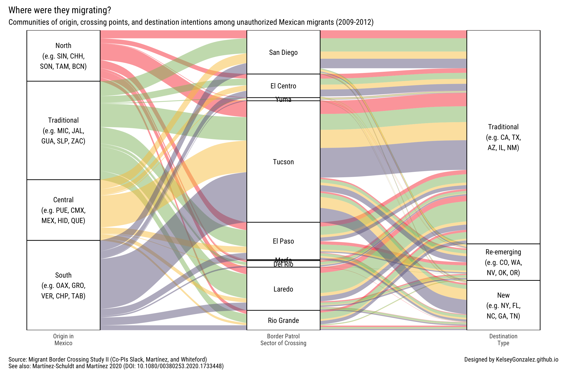
ggsave("featured.png", width = 10, height = 8)Kelsey E. Gonzalez, PhD
Associate Principal Data Scientist
Data Scientist; Computational Social Scientist.